This page contains information about satisfiability (SAT) and maximum satisfiability (MAX-SAT). Although the ideas behind SAT and MAX-SAT are simple I will make them even simpler for all those who are interested in the topic. So here goes...
First, let me be formal in defining it, then I will give examples to clarify things a bit. A SAT expression is composed from a set of m clauses in conjunction,
, where each clause
is formed by the disjunction of Boolean variables,
, or their negation, where
. This form of the conjunction of clauses and the disjunction of literals (variables and their negation) is called Conjunctive Normal Form (CNF). In SAT the problem asks if there exists a truth assignment
such that the expression is true.
What this means is if you have a bunch of variables OR-ed together then you have a clause. If you have several clauses AND-ed together, then you have a formula or an expression that is referred to as CNF formula. Here's an example:
Suppose we have the following variables,
We can create some clauses by ORing variables,
That was simple, now join all these clauses together with AND operators and you will have a formula that looks like this:
where
is the negation of
or not
.
Here's what researchers are concerned about. They are interested in finding out if there exists a
Boolean assignments for each such that
is 1. An example of a satisfying assignment would be:
1
0
1
1
1
When we substitute each of the values of
into
we get,
The result is
= 1. That sounds simple doesn't it? Well it's not. This problem
can be NP-Complete, and NP-Complete problems get harder and harder as the problem becomes larger. So when the number of variables in the formula increase, the problem gets more difficult.
OK, some demystification is in order here. What does NP-Complete mean? I want to make sure that I get this point correctly because my supervisor hates it when I make this mistake. A lot of people think that NP in NP-Complete stands for Non-Polynomial time. This is not true. NP stands for Non-deterministic Polynomial time. What this means is that the problem can be solved with a non-deterministic algorithm, and what's polynomial about it is the verification part. Verifying that the solution provided is a correct one can be done in polynomial time.
Imagine if your boss had a problem that contained 1,000,000 variables and 4,300,000 clauses, and you were asked to find out whether there is an assignment that satisfies the formula. I would suggest that you pack your bags and leave. However, suppose that aliens came to earth and tramped around on their long legged tripods, but instead of herding people into nets and sucking their blood, they solved your problem with their celestially complicated undeterministic machine. You quickly donate a pint of your blood in return for the solution. Now that you have the solution you are faced with something you can easily do: verifying the correctness of the solution. It shouldn't take you very long to show that the solution the aliens gave you does, in fact, satisfy the formula.
Now that we know what SAT is, what is MAX-SAT? MAX-SAT is general form of SAT. In SAT we wanted a decision whether the problem had a satisfiying assignment or not. In MAX-SAT we go beyond that making the problem even harder. The question that MAX-SAT asks is, what is the maximum number of clauses that can be satisfied? This makes maximum satisfiability NP-hard. For one thing, since it's not a decision problem it automatically falls outside the realm of NP-Complete problems. All NP-Complete problems are decision problems. Also, MAX-SAT problems are as hard or harder than SAT problems.
One thing I need to mention before I move on from the NP-Complete realm. When
I mentioned that a SAT problem can be NP-Complete I was trying to say that not
all SAT problems are NP-Complete. A problem that has k variables per
clause is called k-SAT, or MAX-k-SAT. Now, when k
≥
3, then the SAT problem becomes NP-Complete. Otherwise, it is in P, and
therefore easy to solve. With MAX-k-SAT, when k
≥ 2
the problem become NP-Complete. So If boss gave you a SAT problem with k
=
2, your job is still secure.
Applications of SAT and MAX-SAT
So why do we care about this problem?
Really who cares if there is a satisfying assignment or not. SAT and MAX-SAT
problems are more significant than you think. First and foremost, there are real
world applications that depend on finding solutions to SAT problems. Second,
because SAT problems can be represented easily it makes them very attractive to
researchers, and since SAT is NP-Complete that means that if a polynomial time
algorithm was somehow found for it (I doubt it!), then all other NP-Complete
algorithms can be solved the same way. Our friendly blood loving aliens solved this problem a long long time ago, in a galaxy far far away. However, because of their prime directive, "thou shalt not
interfere with internal affairs of other civilizations unless thirsty" means that we have to win the Nobel prize on our own.
The following are some of the applications of SAT:
Electronic Design Automation (EDA) and verification
Automatic Test Pattern Generation
path delay faults
Field Programmable Gate Array routing
Logic synthesis
Crosstalk noise analysis
Functional vector generation
SAT and MAX-SAT Solvers
You will probably not appreciate how difficult an NP-Complete problem such as SAT is until you understand how the solvers work. Suppose your friend, a very naive programmer who flunked his job interview with Google, wanted to take on the SAT problem. He proposed a very simple algorithm: enumerate all possible 1 and 0 configurations, and verify each one. After you smacked him on the head nearly
knocking off his wisdom tooth, you explained that this would work fine for small problems, but as the number of variables becomes large, enumerating all possible combinations becomes impossible. Generally speaking, if you had n variables, then this
exhaustive search requires, at the worst case, 2n tests. For example, if you had 5 variables, then there are 25 = 32 possible configurations: 00000, 00001, 00010, 00011, and so on until 11111. On the other hand, if you had 1000 variables then you need to have,
tests in the worst case to find out if the formula is satisfiable. With 1,000,000 variables there are approximately 10301029 possible configurations. Compare that to the number of atoms in the universe which is only about 1080. That should make your friend
feel ashamed of himself.
Attempting to salvage what's left of your friendship, John
Saturn, your friend rummaged through Google's Scholar for better ideas. This is what he found out. There are two types of search algorithms: complete and incomplete methods. Complete methods perform exhaustive searches. They
guarantee finding an optimal solution if there exists one. However, being complete does not mean checking every possible configuration. They use clever methods to trim the search down. Incomplete methods, on the other hand, do not
guarantee finding a an optimal solution, but if they do find solutions they do it very quickly. They are sometimes
referred to as local or stochastic search algorithms.
Complete Methods
Branch and Bound.
DPL (Davis Putnam Loveland) algorithm.
Branch and Bound
To make life easier, Mr. Saturn, started off
with the simplest complete solver he could get his hands on, Branch and Bound.
It is based on a very simple concept: set a variable to a particular value (0 or
1), apply it to the formula. If that value satisfies all the clauses its in,
then assign a value to the next variable, and so on. If, on the other hand, an
assigned variable unsatisfies one of the clauses, then it is futile to maintain
the state of that variable and assign bits to the rest of the variables. What
this process does is clear. It prunes branches of this large tree that the
different 0 or 1 assignments create. Let's try the following example.
Let's use the formula we started with as an example:
Figure shows the possible assignments each of the variables
through
can
take. So let's start from
with its value being a zero. When we substitute this value into the formula we get a zero in the 2st and 4th clauses, but this does not satisfy
the formula or unsatisfies it. We go to the next variable in the tree, and
that's a 0 for
. When
we plug this value into the formula, then we have the 1st clause satisfied, but
because the 4th clause has both
and
as zeros, then that clause in unsatisfied. Therefore, it doesn't make sense to
continue down that branch for the rest of the variables. That is because there is no way
we can satisfy the formula by applying the rest of the variables,
,
,
or
(think about it or try it for yourself).
We try the second branch of
, and
assign a 1 to it. Now we have satisfied the 4th clause. Traversing the branch
down to
with
0 we get clause 2 satisfied. We keep performing this process until all clauses
are satisfied. Notice that we didn't have to go through every possible branch there is
to the end to guarantee finding the solution or solutions.
Figure : All possible combinations of 0's and 1's for 5 variables.
Although we have reduced the number of checks we performed
it does not mean that the problem has become any easier. It is still hard to solve,
and it is NP-Complete for SAT. Also, this way of pruning the tree applies to SAT
problems, but not MAX-SAT. There is a slight difference that makes the problem
even harder. With MAX-SAT we are not looking to satisfy all clauses. Instead we
want to satisfy the maximum number of clauses, and therefore having an
unsatisfied clause when assigning a particular variable does not mean that we
stop at that point and bound back to the other branch. It could be that
assigning
a 0
unsatisfies a single clause while satisfying many others, and it could be that
if we continue down that branch we get maximum satisfiability. This means that
there are a whole lot more branches that have to be verified. Bounding from a
branch happens only if at any point we find that assigning a value to
yields a greater than or an equal number of unsatisfied clauses than we previously had.
DPL (Davis Putnam Loveland) algorithm
The DPL method is the most commonly used complete method in SAT
and MAX-SAT, and the majority of algorithms created to this date rely on a
modified form of this algorithm. It is basically the same as Branch and bound,
but there is a slight difference which makes it more powerful. The way it works
is this, select a literal (a variable or its negation). Assign the literal a
value. If the literal is true, and hence satisfies the clause, then remove all
clauses containing that literal from the formula. On the other hand, where literal is false due to
its negation, remove only that specific variable from the clause. So far this is sort of
like branch and bound except that we are looking at it from the point of view of
the clauses. We recursively do this until we find a solution. To make this even
better, if a clause contained a single literal, then assign that literal a value
that makes it true, and perform the same procedure. That is called unit
clause elimination. You can imagine how this would have a cascading effect.
As more variables are eliminated from clauses the more clauses turn into unit
clauses. So does DPLL make the problem easier? No. That means that you still have a chance
at being recognised as Nobelaureate if you discover the solution (however
infinitesimally this chance may be).
Here's an example of how DPLL works. Let's start off with our
formula again.
Select
,
and assign a 0 (which makes the clause true). Eliminate the first clause from the formula, and eliminate
from
the 4th clause. This leaves us with the following formula:
Notice now that the third clause in this formula has become a
unit clause. We immediately assign
a 1.
It wouldn't make sense to do otherwise. Now we remove both clauses 1 and 3 from
the formula.
Finally, we set
to 0,
and eliminate it from the formula, and we are left with
.
Setting it to zero satisfies the formula.
There is another trick that was applied to DPLL that was
supposed to improve on the search. It's called pure literal
elimination, but it is omitted from current implementations of the algorithm
due to the limited effect it has. Basically, if a literal appears in a
particular configuration, say
in
all the clauses that the variable appears in, then all clauses containing this
variable can be satisfied by assigning a 0 to the literal. That means that all
clauses containing this variable can be removed.
Incomplete Methods
The fact that complete algorithms still require enormous amounts of time even
on relatively small problems, incomplete methods have been developed to try to
solve the SAT or MAX-SAT problems. Incomplete methods don't guarantee finding
the optimal solution because they don't search the entire space of possible
configurations. They do, however, capitalise on the structure of solution
landscape to converge faster to local or global optimums. A global solution is
an assignment that either completely satisfies a SAT problem, or maximises the
number of satisfied clauses in a MAX-SAT problem. Local optimums are
solutions that the specific incomplete method could not go beyond to find a
better solution.
Incomplete methods are built from stochastic search algorithms such as
GSAT, WalkSAT, Basic Hill-Climbing, simulated annealing, genetic algorithms,
backbone guided, K-Means Clustering, and the list goes on and on. They all have
a random element in their search strategy. The basic premise of these algorithms
is to find the cost (the number of unsatisfied clauses) of random assignments,
and then incrementally adjust these assignments until either a global optimum is
reached in the case of SAT, or time runs out without finding a solution in which
case the algorithm is stopped prematurely. With large MAX-SAT problems it is
unknown if a solution is reached if the formula is not fully satisfiable. Even
that much is not known about the problem.
Here I will discuss the most famous incomplete algorithms namely, GSAT and
WalkSAT. Just as in the case of DPLL, a great deal of the stochastic algorithms
are built on those two.
GSAT
The simplest form of stochastic search is GSAT. It's a very greedy form of
hill-climbing. It starts off with a random assignment and finds its cost. Then
performs a neighbourhood search for the next best cost. The algorithm is as
follows:
Start with a random assignment.
Compute the cost of this assignment.
Find the bit-flip that yield the smallest cost, and flip it.
Repeat from step 3 for a certain number of flips.
Repeat from step 1 for different initial random assignments.
The reason for step 5 is so that if a solution is not found starting from a
particular assignment, then new random starting assignment might lead to a
better solution.
This algorithm, although simple, has been found to be very effective on
problems that DPLL could not manage to solve. However, GSAT very often gets
stuck in local minimums, and even with multiple restarts it plateaus. That is it
reaches a cost that cannot be improved upon even if run for very long. This
where WalkSAT comes into the picture.
WalkSAT
WalkSAT was developed after GSAT. It builds on GSAT by adding a random walk
into the search. It was designed so that with a probability of p GSAT is
performed on the problem, and with a probability of (1-p) a clause that
has not been satisfied is chosen, and a variable that would satisfy the clause is
flipped. That algorithm does much better than GSAT because of the local optimum
escape mechanism, yet it doesn't always solves the problem.
The Complexity of Satisfiability Problems
We've already mentioned how hard SAT and MAX-SAT problems are, but are all
SAT problems equally hard? Extensive studies have been performed on
different problems of relative sizes to understand the complexity and the
structure of the solution landscape. One of these studies found a link between
the hardness of a SAT problem with diluted spin glasses in physics. Then all
hell broke loose, and the physics people got into the game (OK, they might have
been playing this game even before this). All sorts of empirical studies popped
up by the computer science people, and a plethora of theoretical work emerged
from the crazy physics community. I'd stay away from the physics people if I
were you. Unless, of course, you are into sci-fi, the cosmos, and elusively
convoluted theories that only aliens with three legged tripod vehicles can
understand.
It turns out that not all SAT problems are the same. Some problems are harder
than others. Some take a polynomial time to solve, and others grow
superpolynomially and in the worst case even exponentially. It all depends
on the ratio of the number of variables, n,to the
number of clauses, m, in the problem,
.
In order to understand the relationship between the complexity of satisfiability
problems and
there had to be enough SAT problems that can be tested. These were created using
the ever so famous Fixed Clause Length (FCL) model. It's a simple algorithm that created random
satisfiability problem instances that had the same structure as real world
problems. Before I describe the algorithm it's important to remember that when
we
say SAT or MAX-SAT we refer to formulas with clauses that have different a number
of literals in them. The formula we have been using so far was an example of
that. When we say k-SAT or MAX-k-SAT, then we mean
that the clauses contain exactly k literals . Some researchers use k to mean a maximum of k
literals in a clause. We will use
k as a strict number of literals.
How do we create problem instances using the FCL model? The algorithm
works as follow:
Generate m clauses by randomly selecting k
literals from n variables for each clause.
During the selection of the k variables, negate each
variable with a probability of 0.5.
Any repeating clauses are discarded.
Other algorithms were developed before this one, but solving them was easy so
that they were replaced by this one. There also other models that generate even
harder problems, but we won't delve into them. If you are starting off, and
wanted to test your algorithm, I would recommend that you try the problems
available at SATLIB.
They have quite a few small problems that are known to either have fully
satisfiable solutions or they are unsatisfied by a single clause. They also have
some graph colouring problems that were turned into SAT problems.
The Complexity of SAT and MAX-SAT problems
Now that we know how a problem is generated, and we already mentioned that
the difficulty of the problem is related to
let's understand what it means to have an easy-hard-easy transition for SAT
problems. Then we will talk about the complexity of MAX-SAT. A few researchers
generated thousands if not millions of random SAT problems. They varied the
ratio
of the problem from 0 to a 10 or 20. So imagine that the number of variables
they started with was 100, they varied the number of clauses from 0 to 1000.
Then they applied the famous DPLL algorithm to these problems. They either used
time as a measure of complexity to see how long it takes to find a
solution, or they resorted to the number of flips (which is the most common
one). What they noticed was that as
increased from 0 to 4.3, the problem started off easy, requiring a small number
of flips to find a solution, to hard, requiring significantly more flips, and
then to
easy again after
= 4.3. The point where
= 4.3 is called the phase transition point. A rough sketch of this phase
transition is shown with the red curve in Figure .
That's the easy-hard-easy transition. The blue curve relates the percent of fully satisfiable problem instance in relation to
.
You can see that at the phase transition one-half of the problem instances are
fully satisfiable. Below the phase transition, the majority of the problems are
satisfiable, and above it the majority are unsatisfiable.
Figure : The
relationship between the and the number of flips required to
find solve the problem (red). The percent of fully satisfiable problem
(blue). This figure was created based the graph in the paper,
"Experimental results on the crossover point in random
3-SAT."
What's going on here? Why is the problem easy at first, and then
difficult? What's even more strange is that the problem become easier to
solve afterwards. Why is that? The reason is hidden in the structure of the SAT
problems. When a problem instance is below the phase transition, it contains many
solutions, and hence does not require a great deal of search to find one of
these solutions, however as the problem reaches the crossover point (at the
phase transition), then the problem contains many almost-satisfiable solutions.
This means that the search algorithm has to go deep into the search tree before
it discovers that a solution does not exist. In other words it has large and
deep plateaus of almost-satisfiable solutions that require the DPLL to perform
a great deal of checks. After the phase transition the fully satisfiable
solutions are reduced even further, but this time DPLL doesn't have to go too
deep to discover that a solution does not exist, and a great many parts of the
tree are pruned at the top of the tree. This reduces the complexity of the
search again.
In MAX-SAT this relationship holds true before the phase transition,
but then problems become difficult and stays difficult even after the transition
point. This is known as an easy-hard transition. The reasons
mentioned for the SAT problem hold for the MAX-SAT problem before the
phase transition. However, remember that we are not testing for satisfiability
here. We don't prune the tree as soon as we find an unsatisfied clause. In this
case, the search tree has to be traversed until a worst or equal cost is found, then we
prune. That means that there are a lot more depth searches than there are for
SAT problems. That's why MAX-SAT is NP-Hard rather than NP-Complete. It is as
hard as a SAT problem and even harder.
What happens when we use incomplete algorithms to find
solutions? We have found that for MAX-SAT problems a stochastic search has an
easy-hard-easy transition even for local optimums. This is a very important
result. It shows that even stochastic searches find the a satisfiability problem
difficult, but it's only when n is large enough that we get to see the
effect that a problem has on incomplete methods. Lots of the research with
complete algorithms was done on small problems. These problems, however, are
easy for incomplete algorithms. Only when the tests were carried on larger
problems that these difficulties were hit in almost the same way.
The Structure of the Solution Space
The complexity of satisfiability problems gave us insights into
the structure of the solution space. However, the insights were nothing more
than an imaginative picture. There was no solid evidence into how things really
looked. Further research was performed on the relationship between the different
local and global optimums. The solution landscape began to decloak, and the
picture got more interesting, and much more useful.
Using the Hamming distance between local and local, and local
and global optimums it was shown that the local optimums with better costs
were closer to the global optimums. So the better the cost of a solution, the
closer in Hamming distance it is to the global optimum on average. In fact,
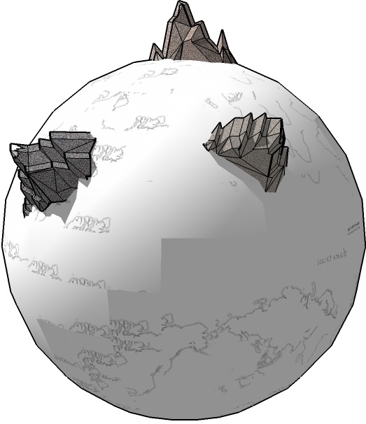
further studies have shown that the global and local solutions formed clusters
in space. So imagine the solution landscape as a hemisphere with many different
hills. The highest peaks of some of the hills represent global solutions. The lower
peaks represent the local solutions. If you were to look at the mountains from
afar you would see this gradual increase in peak height. The mountain would
take on this rough pyramid or cone shape. However, if you get closer to a
particular mountain, then you would see that the highest peak is not necessarily
the centre of the mountain nor are the smaller peaks the closest to global peak.
Roughly speaking or on average they are. A 3-D schematic of this concept is shown in
figure . This more like a 2-D image of a
3-D projection that is supposed to represent an n dimensional {0, 1}
space. Which is probably not a great representation, but it'll do.
Figure : The landscape
of solutions of satisfiability problems. Each mountain is
like a cluster of local and global optimums with better cost solutions
closer to
global optimums.
Since the local optimums shared some of their truth assignments with global
optimums, local optimums were used to locate the global optimums. One of the
methods used to find global optimums from information found in local ones is
called Backbone Guided Local Search. Consider the truth assignments (a string of
0s and 1s) that make up all the global solutions. Although they might be
different in some parts of the their makeup, but they have a great deal of
commonality. These common traits (bits in this case) make up the backbone of the
solution. Since the backbone is also shared with local solutions, the search
algorithm that was designed for this sort of thing built the backbone
stochastically. The reason I say stochastically is because the backbone of the
solution is not known. If it had been, then the solution would be easily found.
So the algorithm goes around searching for this backbone, and if certain bits
appear more frequently than others, then it is more likely that they are in the
backbone.
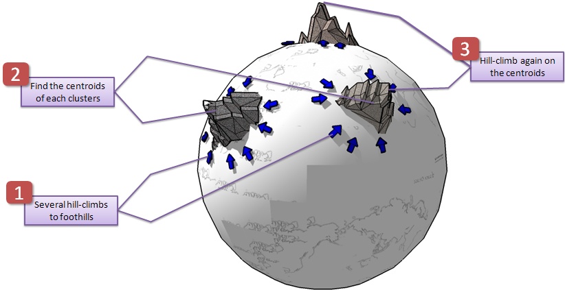
Another method that we have developed to
capitalise on this picture is Hill-Climbing/K-Means algorithm search. K-Means basically groups
similar assignments in clusters, and finds their centres or centroids (as the
Vector Quantization community would like to call them) .
We were able to jump closer to
the peaks of these mountains very quickly. Thus, we were able to locate better
solutions more effectively. We start off with a basic hill-climber from
different initial random assignments. Then we cluster these assignments using
the K-Means algorithm. In effect we group the assignments of the different
mountains together. Then we take the centroids of these clusters, and apply
hill-climbing on them a second time, Figure
. This scheme gave us really good results
with large satisfiability problems. Not only do we show that this works, we also
performed a great deal of analysis to "prove" our case. You can find more in-depth
analyses in Learning
the Large-Scale Structure of the MAX-SAT Landscape Using Populations paper
published in the IEEE transactions on Evolutionary Computation.
Figure : To find better solutions more efficiently, perform
several quick hill-climbs to the foothills, then cluster
the solutions using K-Means. Use the centres of the clusters for further
hill-climbing.
Further Reading
If you are interested in knowing more about the problem you can try the
following links:

 , where each clause
 is formed by the disjunction of Boolean variables,
 , or their negation, where
 . This form of the conjunction of clauses and the disjunction of literals (variables and their negation) is called Conjunctive Normal Form (CNF). In SAT the problem asks if there exists a truth assignment
 such that the expression is true.


 is the negation of
 or not
 such that
 is 1. An example of a satisfying assignment would be: